NeRF from Scratch!

In this project, we are implementing Neural Radiance Fields, or NeRF, from scratch! In part 1, we are training a neural network to predict rgb values based on 2D coordinates. This is just to get us warmed up for the actual radiance fields in 3D.

Part 1

Architecture

We followed this architecture, which includes positional encoding, and linear layers followed by ReLU activation functions, and a sigmoid function at the very end.

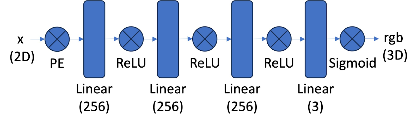
The positional encoding expands the input dimensions by creating more channels with sinusoidal functions. L defines the maximum frequency in the sinusoidal functions. For example, a 2D coordinate in this case with L = 10, becomes dimensions + 2 (for sin and cos) * L * dimensions = 2 + 2 * 10 * 2 = 42.

Here is the PE function:

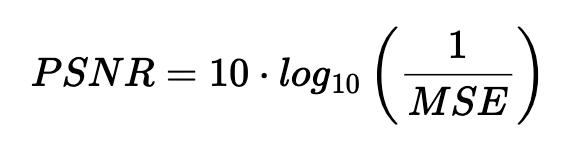
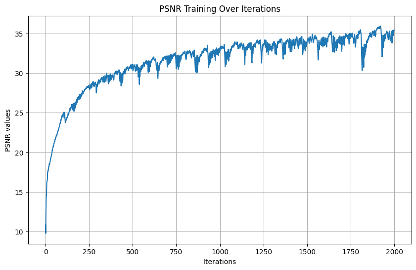
In training, Peak signal-to-noise ratio (PSNR) is a good metric to assess the reconstruction of an image. The higher the PSNR, the better – the more signal and less noise. PSNR is defined as follows:

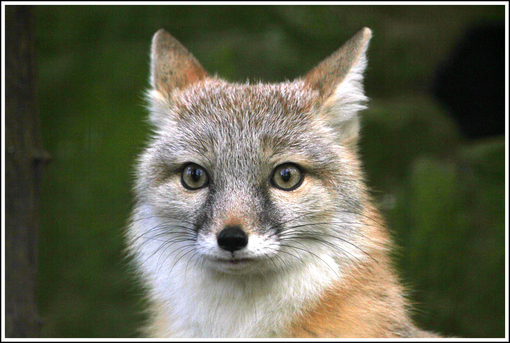
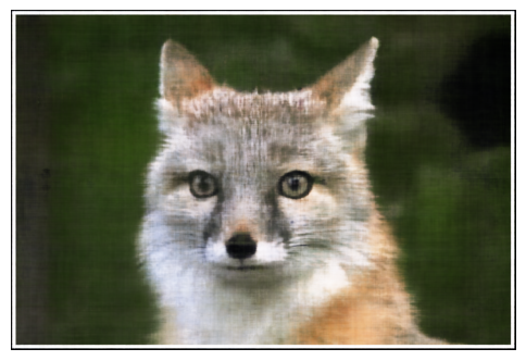
Original fox image

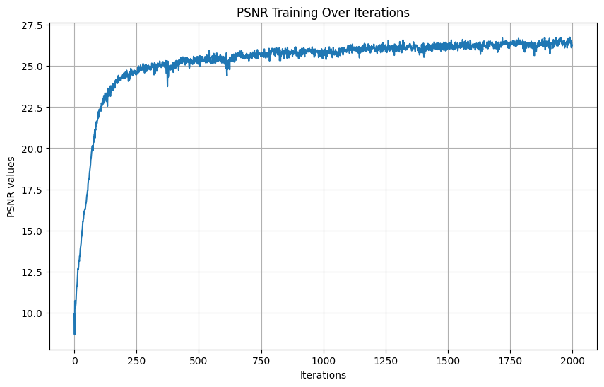
PSNR Curves

First one:

Learning rate: 1e-2
Batch size: 10000
Num iterations: 2000
L: 10

Tried different hyperparameters

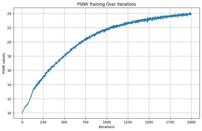
Changed the learning rate to 1e-4:

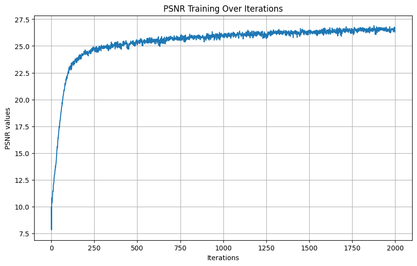
Doubled L (max frequency for PE) to 20:

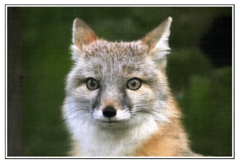
Results: Fox over different iterations: [0, 500, 1000, 1500, 1999]

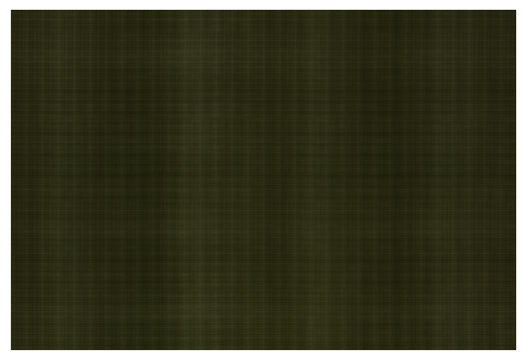
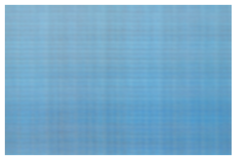
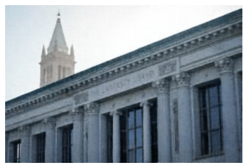
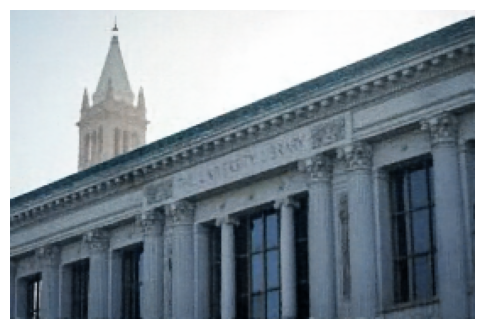
Now we’ll do this on an image of our choosing– an image of Doe library (where we mainly worked on this project).

This tuning really depends on the image– here’s Doe at the last iteration with:

Learning rate: 1e-2
Batch size: 10000
Num iterations: 2000

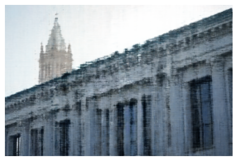
Not so great

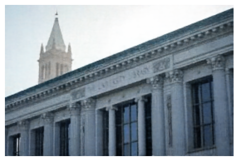
But now, we will change L to be 7 for 3000 iterations, and it is much better. This reflects the role the added dimensionality the positional encoding provides, and in this case reducing L and therefore the added dimensionality helped with the final result.

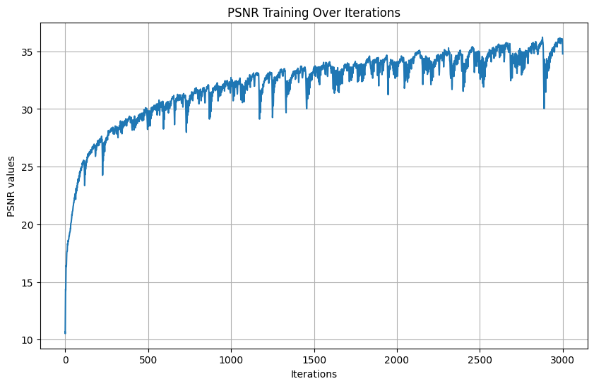
Doe over different iterations: [0, 1000, 2000, 2999]

Part 2

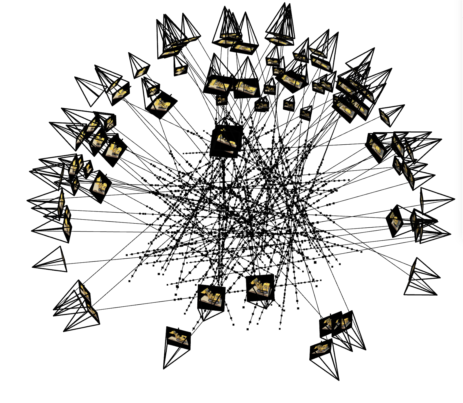
Okay, this 2D network was just warm up– now onto NeRF. NeRF aims to learn a neural network that transforms 3D points in space and viewing directions into RGB colors and density values. These outputs allow us to render photorealistic images of a scene from any perspective. The data we have is the multi-view calibrated image data of a lego truck, taken from the original NeRF paper (except in lower resolution). This includes the camera - to - world transformation matrices. We implemented a function pixel_to_ray (and a couple helper functions) to transform pixel values into ray origin and ray direction vectors, using the camera’s intrinsic matrix and the camera-to-world matrices we have. We sampled a fixed number of rays per image (so if you define 10,000 rays and there are 100 images there would be 100 rays per image for example). Then, we sampled points along these rays. Note that to avoid overfitting these points along rays were not uniformly distributed–instead we added random, small perturbations. This is the plot of cameras, rays, and samples in 3D–pretty cool!

3D Camera Visualization

NeRF Architecture

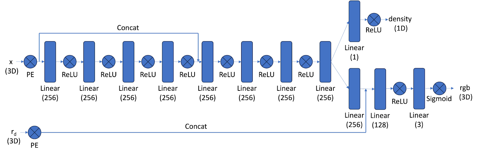
We implemented a NeRF architecture that builds upon the principles discussed earlier. PE is the same as defined in part 1, but instead is fed 3D spatial coordinates instead of 2D, and ray directions are transformed into a higher-dimensional space to enable the network to capture variations in the scene. The network itself is significantly deeper, consisting of many repeated linear layers. This depth allows the model to effectively learn the intricate relationships between geometry and appearance within the scene. The inputs to the network are the 3D coordinates of the points sampled along each ray and the directions of the rays. The outputs are density, which describes the opacity or how much light is absorbed or scattered at each sampled point, and the RGB color values. Finally, we implemented a volume rendering function to synthesize the final pixel colors. This function integrates the predicted densities and RGB values along each ray to render photorealistic views of the scene. We used the following discrete approximation equation for rendering.

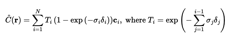
sigma is density, c is color, and delta is the interval width between points on a ray. Due to memory errors, we were only able to make our batch size 1000– 1000 rays total per iteration. We ran for 5000 iterations, with a learning rate 5e-4. This took about 20 minutes. We were able to surpass the required PSNR of 23. If we had more compute units, we could have increased batch size and iterations to further increase performance. T This is the actually the validation PSNR curve (it says training but that is an incorrect title).

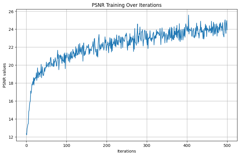
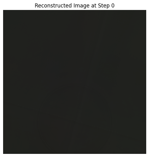
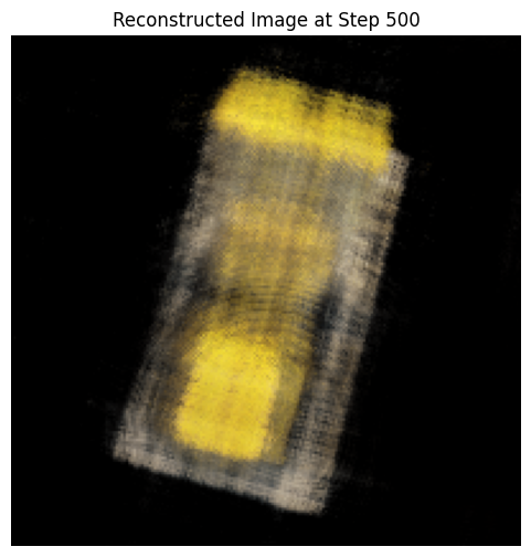
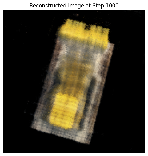
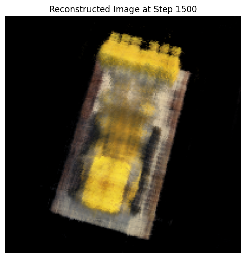
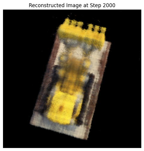
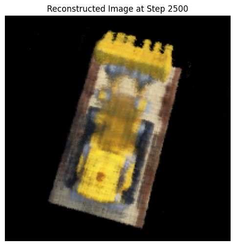
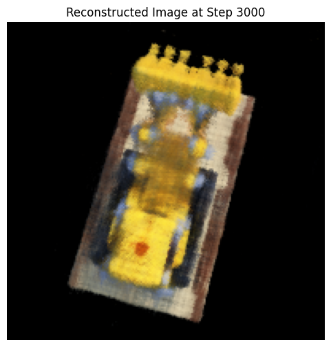
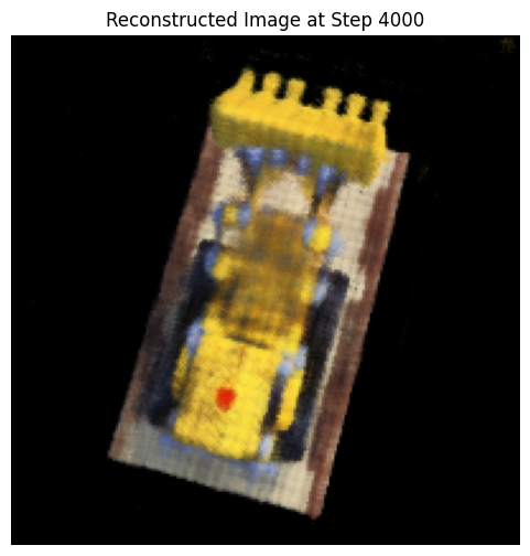
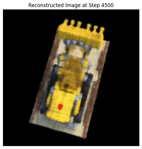
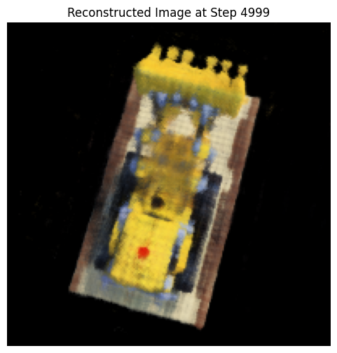
These are novel view images (top view) at different iterations.

This is the reconstructed spherical view from the test set camera-to-world matrices.

Bells and Whistles

In order to change the background color of this rendering, we can inject color into the volume rendering. We did this by creating a new volume rendering function that includes background color as a parameter. The function modifies the normal volume rendering process to account for a background color by adding an additional step at the end. In standard volume rendering, the final color is calculated by summing the contributions of each sampled point along the ray. To include the background color, the function computes the remaining transparency of the ray (i.e., 1−sum of contributions from the scene) after accounting for all sampled points. This remaining transparency is then multiplied by the background color and added to the rendered scene colors.